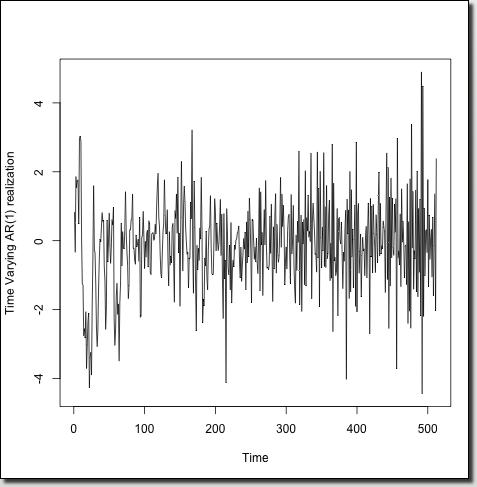
Simulated Autoregressive Example

The figure on the left shows a realization of a time-varying autoregressive process (TVAR for short) of order 1. This is similar to the (stationary) AR process introduced in the introduction: the crucial difference being that in the TVAR(1) process the constant parameter a is permitted to change over time and become at. In other words the model behind the TVAR(1) is

x_t = a_t x_t-1 + z_t.

For the figure the parameter a_t varies linearly from 0.9 to -0.9 over the extent of the series.

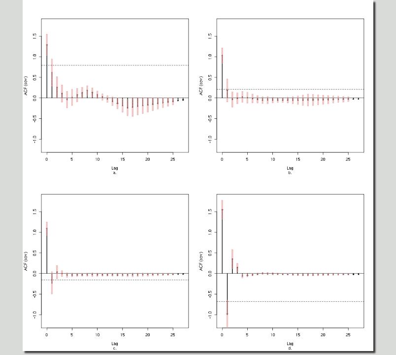
Localized Autocovariance

Figures a., b., c. and d. below are the localized autocovariances of the simulated series at times 100, 200, 300 and 400 respectively. One can clearly see how the process behaves like an AR(1) process with positive a near to the left of the plot and this is reflected nicely in the localized autocovariance in Figure a. below. Similarly, the process behaves like AR(1) with a negative a near to the right of the plot, and this is reflected in Figure d. Figures b and c show what is going on near to times 200 and 300.

Plot (a.) shows the localized autocovariance around time 100. The TVAR(1) parameter around this time point is about 0.55 and the true autocovariance for an (equivalent stationary) AR process is about 0.79. The dashed horizontal line is drawn at height 0.79 in plot (a.) and it can be seen that the 95% CI for the lag one autocovariance covers it. Similarly, for the other three plots the 95% CI cover the true values of the parameters at lag one.

It is certainly useful to compare the true values with the estimates but it it also useful to take in all four pictures as a whole. The localized autocovariance plot at time 100 (a.) looks like the autocovariance for an AR process with positive mid-sized parameter, and the plot at time 400 (d.) looks like the autocovariance for an AR process with negative mid-sized parameter. As a whole one can see the TVAR parameter changing from positive to negative in the single realization , i.e. a nonstationary realization

FTSE Localized Autocovariance>.