Stationary Models

In this short article we do not have the time and space to give a full treatment of statistical models. However, we briefly describe one model here in layman's terms. A time series model explains how time series values evolve from one time step to the next.

For example, in words we might say:

The value now = Roughly the value previously + some random disturbance

This is the well-known random walk model.

Mathematically, the model can be written as:

x_t = a x_t-1 + z_t

This should be read as: “the value of the series at time t is equal to a times by the previous value of the series (at time t-1) plus some noise”. Here the z_t quantity is independently distributed random noise. This model is called an autoregressive model of order 1 and this is abbreviated to AR(1). (You might imagine that higher orders would involve x_t-p for p>1 and you'd be right).

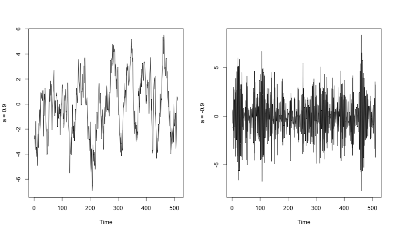
The behaviour of an AR(1) process depends very much on the value of the parameter a. In the left plot below is a realization of an AR(1) process with parameter a=0.9. Here, consecutive values of the time series are reasonably similar so that the process does not oscillate quickly. The right plot shows a realization of an AR(1) process with parameter a=-0.9. Here, consecutive values are dissimilar and the process oscillates wildly around the mean value (which is zero in both cases).